Compute expectation and covariance of Brownian bridge
Let $\{X(t), t \geqslant 0\}$ be a standard Brownian motion. That is, for every $t \gt 0$, $X(t)$ is normally distributed with mean $0$ and variance $t$.
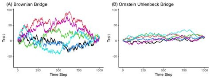
Then $\{X(t), 0 \leqslant t \leqslant 1 | X(1) = 0\}$, known as the Brownian bridge, is a Gaussian process. That is, for every $0 \lt t \lt 1$, it is multivariate normally distributed.
Thus, I want to find its the marginal mean values and the covariance values.
Remark) There is two true equations. $$\tag{1} E\left[X(s)|X(t)=B\right]=\frac{s}{t}B$$ $$\tag{2} \text{Var}\left[X(s)|X(t)=B\right]=\frac{s(t-s)}{t}$$
- For $s\lt1$,
$$E\left[ X(s) | X(1) = 0 \right] = 0$$
- For $s\lt t\lt 1$,
\begin{align} \text{Cov}\left[ \left(X(s), X(t)\right)|X(1)=0\right] &= E\left[ X(s) X(t) | X(1) = 0 \right] \\ &= E\left[E\left[ X(s) X(t) | X(t), X(1) = 0 \right]|X(1)=0\right] \tag3\\ &= E\left[X(t) E\left[ X(s) | X(t)\right]|X(1)=0\right] \tag4\\ &= E\left[X(t) \left.\frac{s}{t} X(t)\right|X(1)=0\right] \quad \text{by (1)}\\ &= \frac{s}{t}E\left[\left.X^2(t) \right|X(1)=0\right] \\ &= \frac{s}{t}\cdot t(1-t) \quad \text{by (2)}\\ &= s(1-t) \end{align}
I cannot understand equation $(3)$ and equation $(4)$ are derived.
Please give me some explanations with a detailed process.
Thank you for reading my question.
$\endgroup$ 33 Answers
$\begingroup$In equation (3), Let $E_1$ denotes the conditional expectation$E(|X(1)=0)$ we use the iterated expectation , that is $E_{1}(X(s)X(t))=E_{1}(E(X(s)X(t)|X(t))$.
In equation (4), since we conditioned to X(t), that means that we know its value , hence X(t) is not random anymore under that assumption: we can remove it from the expectation term as if it was deterministic.
$E_{1}(X(s)X(t))=E_{1}(X(t)E(X(s)|X(t)))$
$\endgroup$ 3 $\begingroup$The explanation contains some errors so I will start at the beginning. $[X]$ is the distribution of the random variable, $X$. $[X | Y]$ is the conditional distribution of $X$ given $Y$.
Let $(W(t): t\geq 0 )$ be standard brownian motion.
$[W(s) | W(t) = y] = P( W(s) \in dx, W(t) \in dy ) / P( W(t) \in dy)$
$=P( W(t) \in dy | W(s) = x ) P(W(s) \in dx)/ P( W(t) \in dy)$
$=\frac{1}{\sqrt{t-s}} \phi\left(\frac{y-x}{\sqrt{t-s}}\right) \frac{\frac{1}{\sqrt{s}}\phi(\frac{x}{\sqrt{s}})}{\frac{1}{\sqrt{t}}\phi(\frac{y}{\sqrt{t}})}$
Completing the square in $x$ gives
$\sqrt{\frac{t}{s(t-s)}} \phi\left(\frac{x - \frac{s}{t}y}{\sqrt{s(t-s)/t}}\right)$
Now the mean, variance and second moment are straightforward:
$\mathrm{E}\left[ W(s) | W(t) = y\right] = \frac{s}{t} y$
$\mathrm{var}\left[ W(s) | W(t) = y \right] = \frac{s(t-s)}{t}$
$\mathrm{E}\left[ W(s)^2 | W(t) = y\right] = \frac{s(t-s)}{t} + \frac{s^2}{t^2} y^2$
Finally the covariance. Assume $ r < s < t $ :
$\mathrm{cov}\left[ W(r), W(s) | W(t) = y\right]$
$=\mathrm{E}\left[W(r)W(s) | W(t) = y\right] - \frac{r s y^2}{t^2}$
Continuing with the cross moment in the first term above,
$\mathrm{E}\left[W(r)W(s) | W(t) = y\right]$
$= \mathrm{E}\left[\mathrm{E}\left[W(r)W(s) | W(s), W(t) = y\right] | W(t)=y\right]$
$= \mathrm{E}\left[\mathrm{E}\left[W(r)W(s) | W(s)\right] | W(t)=y\right]$
$= \mathrm{E}\left[W(s) \mathrm{E}\left[W(r)| W(s)\right] | W(t)=y\right]$
$= \mathrm{E}\left[W(s) \frac{r}{s} W(s) | W(t)=y\right]$
$=\frac{r}{s}\left[\frac{s(t-s)}{t} + \frac{s^2}{t^2} y^2\right]$
In the above, the first equality follows, as someone pointed out above, by the iterated expectations, e.g. $\mathrm{E}[ \mathrm{E}[ Y | X ] ] = \mathrm{E}[Y]$. If the outer expectation is conditional as well, everything is conditional upon that: $\mathrm{E}[ \mathrm{E}[ Y | X, W ] | W] = \mathrm{E}[Y | W]$. The next equality follows because $W(r)$ and $W(t)$ are independent given $W(s)$ because of the Markovian property of brownian motion. The next equality follows because we can pull $W(s)$ out of the inner conditional expectation, because, conditional upon it, it is a constant. The next equality is the above result regarding the mean, and the final equality follows from the above result regarding the second moment.
Having computed the cross moment, we can plug its value back into the above expression for the covariance. After simplifying, we obtain:
$\mathrm{cov}\left[ W(r), W(s) | W(t) = y\right] = \frac{r(t-s)}{t}$
The mean, variance, and covariance function for brownian bridge now follow if we replace $(r,s,t,y)$ with $(s,t,1,0)$.
$\endgroup$ $\begingroup$As you well stated, the Brownian bridge is a GP. That means that given training outputs $f$ and test outputs $f_{\star}$the joint prior distribution is
$$\begin{bmatrix}f\\f_{\star}\end{bmatrix} \sim N \Bigg(0, \begin{bmatrix}K(X,X) & K(X, X_{\star})\\K(X_{\star}, X) & K(X_{\star}, X_{\star})\end{bmatrix}\Bigg) \tag{1}$$
where $X$ and $X_{\star}$ are the training and test inputs respectively. If there are $n$ training points and $n_{\star}$ test points then $K(X,X_{\star})$ denotes the $n \times n_{\star}$ matrix of the covariances evaluated at all pairs of training and test points, and similarly for the other entries $K(X, X)$, $K(X_{\star}, X_{\star})$ and $K(X_{\star}, X)$. Each covariance corresponds to the Wiener process:
$$k(x,x’) = \min(x,x’) \tag{2}$$
To get the posterior distribution over functions you need to restrict this joint prior distribution to contain only those functions which agree with the observed data points, corresponding to conditioning the joint Gaussian prior distribution from eq. (1) on the observations, i.e
$$f_{\star}|X_{\star}, X, f \sim N \big(K(X_{\star}, X)K(X,X)^{-1}f, K(X_{\star}, X_{\star}) - K(X_{\star}, X)K(X,X)^{-1}K(X,X_{\star})\big) \tag{3}$$
(See, e.g. von Mises [1964, sec. 9.3] for this deduction)
In our case:$X = \begin{bmatrix}0\\1\end{bmatrix}$ and $f = \begin{bmatrix}0\\0\end{bmatrix}$
if you compute the covariances from eq. (2) and replace them in the posterior covariance of eq. (3) you get the desired output:$\text{cov} (x,x’|x(t) = 0) = \min(x,x') - \frac{xx’}{t}$
in particular, for the variance ($x=x’=s$) you have:$\text{var} (s|x(t) = 0) = \frac{s(t-s)}{t}$
Caveat: $K(X,X)$ is singular given the training points, to compute $K(X,X)^{-1}$ you can add noise $\sigma^{2}$ to the model and then compute the limit when $\sigma \rightarrow 0$. The equivalent eq. (3) with noise is obtained by doing the following replacement:$K(X,X) \rightarrow K(X,X) + \sigma^{2}I$
$\endgroup$