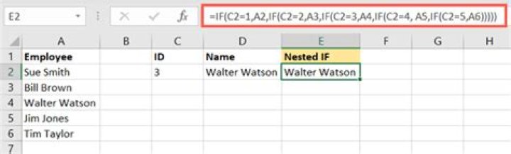
Excel find bucket without nested IFs
I have to separate my data in category, say for example:
Category Minimum Maximum A -100 -20 B -20 0 C 0 +20 D +20 +100So if one data point is -50, it belongs to Category A.
One solution is to use nested IFs:
=IF(A1<-20,"A",IF(A1<0,"B",IF(A1<20,"C","D")))But when the number of categories increases it becomes quite messy. Is there a better way to achieve the same?
3 Answers
Assuming you have the table with categories in Y2:Y10 and the minimums in Z2:Z10 (with 20 not +20 and similar for all positive numbers) then you can use a LOOKUP formula
=LOOKUP(A1,Y$2:Y$10,Z$2:Z$10)
Assumes there are no gaps in the ranges, i.e. the maximum for each category is effectively assumed to be immediately beow the next minimum
2Another solution could be using named ranges.
I would modify your example to this:
Category Minimum Maximum
Cat_A -100 -20
Cat_B -20 0
Cat_C 0 +20
Cat_D +20 +100
Then mark the data from Cat_A to +100, and use Make from selection (On Formula Tab, Section Defined Names) - use make from left column.
The you will get 4 named ranges Cat_A, Cat_B, Cat_C and Cat_D, which you can use in your workbook for i.e. conditional formatting, unsing Min(Cat_A) and Max(Cat_A) as limits.
However, this solution is more an extention to the one of barry houdini.
I use this trick for equal data bucketing. Suppose you have data in A1:A100 range. Put this formula in B1:
=MAX(ROUNDUP(PERCENTRANK($A$1:$A$100,A1) *4,0),1)Fill down the formula all across B column and you are done. The formula divides the range into 4 equal buckets and it returns the bucket number which the cell A1 falls into. The first bucket contains the lowest 25% of values.
Adjust the number of buckets according to thy wish:
=MAX(ROUNDUP(PERCENTRANK([Range],[OneCellOfTheRange]) *[NumberOfBuckets],0),1)The Advantage
The advantage of this solution is that you do not have to worry about the min and max of each bucket. The min and max parameters will mysteriously adjust themselves keeping equal number of observation in each bucket.